Organisation of data
Contents
- Data structure definition
- Static and dynamic data structures
- 1D Arrays
- 2D arrays
- Linked lists
- Stacks
- Queues
- Matrices
Data structure definition
In computer programming, a data structure is a predefined format for storing, accessing, and processing data in a computer program.
Unlike a data type, which defines a way to hold a piece of data, data structures are designed for holding multiple pieces of data in a structured way.
Static and dynamic data structures
This isn’t explicitly on the spec, but it’s great to know anyway.
When you store data in memory, you need to decide if it’s static or dynamic.
Static
An example of static data would be an array.
When you create an array, you tell the compiler how big you want it to be. When the program is executed, it will reserve enough memory for the size you’ve specified. It never expands or shrinks.
You cannot change the amount of memory reserved for the array while being run.
Static data types can cause issues:
- if you end up trying to save/read from higher memory addresses than you’ve reserved, the program will crash
- if you reserve too much memory, you’re being wasteful
Dynamic
Dynamic variables don’t have a fixed size in memory. An example of this is linked lists.
With linked lists, each item has a pointer to the memory address where the next item in the list can be found.
When you add more items to the list, more memory is allocated. Dynamic data is much easier to work with because of this.
Queues and stacks are examples of dynamic data structures, which we will learn about later in this document.
1D Arrays
Arrays are containers which can be used to store a specific amount of a data type (a way to define how data should be interpreted and transformed from its binary representation).
For example, you might have an array of integers for storing a list of a class’s test scores.
Arrays can be thought of as lists. An array is initialised with a size, which is the maximum number of values (called elements) which can be contained in it.
Arrays are immutable in most languages as the number of items they store cannot increase or decrease at runtime. This means that, after it’s set, it cannot change.
The elements in the array can then be accessed using an index. Accessing the array with an index (usually like arrayName[index], such as scores[3]) provides the value at that position in the array.
Indexes are usually 0-indexed in most languages, meaning an index of 0 provides the 1st value, and in index of 1 provides the 2nd value.
Storing arrays in memory
The array variable stores a value called a pointer. This pointer points to the memory address where the array begins.
In low-level languages, this is why accessing an array variable without an index provides a number: this is the address in memory where the array data is stored.
Diagram showing how 1D arrays are accessed in most languages
2D arrays
A 2D array is literally just an array of arrays! It’s easiest to think of them as tables.
For example you might use a 2D array of integers to store a class’s scores per question in a test (studentScores):
| Q1 | Q2 | Q3 | Q4 | |
|---|---|---|---|---|
| Student 1 | 3 | 2 | 4 | 1 |
| Student 2 | 4 | 3 | 1 | 2 |
| Student 3 | 1 | 0 | 2 | 5 |
You’d access the array of student 1’s results using studentScores[0], and student 1’s Q2 result using studentScores[0][1].
Linked lists
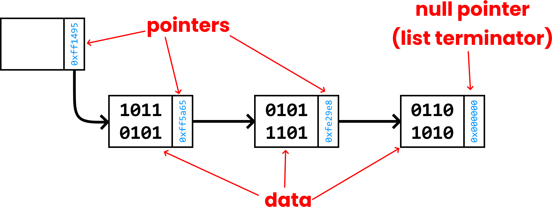
Linked lists are mutable (changeable) collections of items that grow and shrink as needed. They are mutable as the number of items in them can increase or decrease at runtime.
Data in a linked list is not stored in a single block of memory. Instead, each node of the array contains the data for that node, and a pointer to the address in memory which stores the next node.
This allows the list to expand as needed as more nodes can be added by setting the memory address in the previous node. This also allows for nodes to be inserted mid-list.
The pointer at the start node in a list is called the starting pointer. This points to the first piece of data in the list.
The pointer at the last node in a list is null (all zeroes).
Example of a linked list
Stacks
Stacks work on the “last in, first out” system (LIFO): the last item to be put into a stack is the first item to be popped out.
With a stack, you can only access the first item (at the top). Think about a stack of plates: you wouldn’t take a plate from the middle of a stack, you’d take it from the top.
Adding an item to a stack is called pushing it onto the stack. Removing an item from a stack is called popping.
Stacks are allocated memory dynamically: the grow and shrink as needed.
A stack of plates!
Please remember that the idea of a “stack” of items on top of each other is a way for humans to think of it. It’s not stored like this in memory, but is instead programmed to behave like this.
Push and pop excercise
Create a stack capable of holding 6 integers.
- Push 5, push 3, push 4, pop, push 2, pop, pop, push 1
- Push 1, push 2, push 3, push 4, push 5, pop, pop, pop, pop, pop
- Push 7, push 3, pop, pop, push 1, pop, push 7, push 8, push 9, push 11, push 12, push 8, pop
Answers
1- None - it’s empty
12
Cheeky trick - you don’t need to look at the whole stack. Instead, you can work your way backwards. For 1, it ends with a push of 1, so you can be sure 1 will be at the top of the stack.
For 2, you can count the pops going backwards, then ignore that amount of pushes. There are 5 pops, so we ignore 5 pushes. We’re left with nothing.
For 3, we pop once, so we go backwards and ignore the first push, so we finish with the 2nd to last push, which is 12.
What are stacks actually used for?
A great example of where stacks are used is during interrupts. Before an Interrupt Service Routine (ISR) is run, the CPU will push the values from all the CPU registers into a stack. Once this ISR is complete, the values are popped off to continue execution where it left off.
Another place that stacks are used is programming. When you call a function, the address you were running instructions is pushed onto a stack so that the program knows where to continue execution when the called function finishes.
Queues
Queues work via a “first-in first-out” (FIFO) or “last-in last-out” (LILO) system: the first item added will be the first item removed.
We use the same words push and pop to describe the adding and removing of data, but we also use enqueue and dequeue.
Both the front (head) and end (tail) of the queue is visible at all times.
Queues are also dynamic: they grow and shrink in size as items are added and removed.
Questions
Set up a queue which holds 5 integers. What values are left in the queue and what are the items that have been removed.
- E5, E7, E10, D, D, E1, D
- E1, E2, E3, E4, E5, D, D, D, D, D
- E3, E8, E9, D, E7, E2, E12, E1, D
Answers
- In queue:
1. Removed:5,7,10 - In queue: none. Removed:
1,2,3,4,5 - In queue:
9,7,2,12. Removed:3,ERROR: FULL,8
Where are queues actually used?
Printers! When we queue something for printing, jobs are completed in the order they are sent. Otherwise it would be a little unfair to the poor person waiting for their print job.
Media streaming. When you watch video, the stream is played in the order the chunks are received. You wouldn’t want it skipping ahead, then playing backwards.
Matrices
A matrix is a mathematical construct for a table of numbers, usually represented as an array in computing. In computing, we store matrices as 2D arrays.
A matrix’s size is represented by its dimensions (also known as its order). These dimensions are represented by RxC, where R is the number of rows and C is the number of columns.
Be warned! You might be used to referring to dimensions as width x height. Matrices are the opposite!
1  7
5  3
2  8
This matrix would have the dimensions 3x2.
Matrices vs Arrays
Arrays can be any number of dimensions: you can have 1D (a single collection), 2D (like a matrix), 3D (like an array of tables).
Matrices are a fixed table construct: 2D only, with a fixed count of rows and columns.
Matrices only have numbers!
Accessing data in matrices
To access data in a matrix, we need to use two indices: one to show the row, and the other to show the column. These two indices then allow us to find the one item of data in that position.
The first index is the row number, and the second index is the column number. This is called row-major ordering as the row index comes first.
For example [4, 2] (zero-indexed) is the 5th row, and 3rd column.
Matrix as 2D array example
| 4 | 2 | 1 | 3 | 5 |
| 7 | 9 | 10 | 7 | 8 |
| 14 | 13 | 15 | 11 | 12 |
[0, 3]-3[2, 2]-15[1, 4] x [2, 1]-8 x 13=104
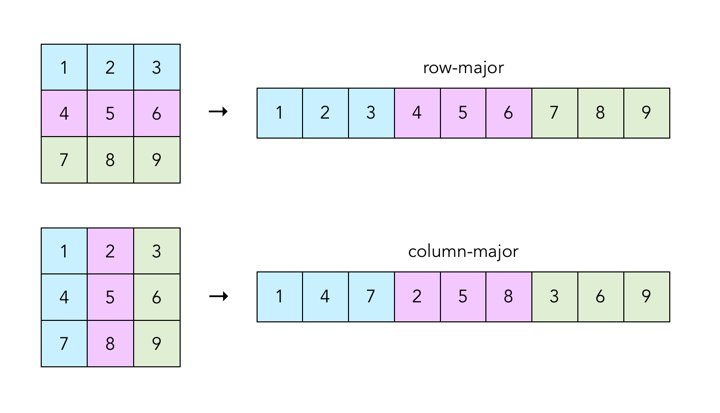
Storing matrices - column-major and row-major
There’s two different ways to represent matrices: row-major order or column-major order.
In row-major, we store the matrix contents one by one, starting with the first row, moving between values from left to right, then to the next row. These values are stored next to each other in memory.
In column-major, we go down the columns first, and then move to the next row.
A diagram showing the difference between row-major and column-major ordering.
In an exam, you might be told an ordering method, and be given an array/matrix, and asked for the value at a certain index in memory.
Matrix mathematics
You might be asked to perform different mathematical operations on matrices.
Addition

In this example, two matrices are being added together.
For addition, we simply layer the matrices on top of each other, and add the two values.
For example, to work out the top-left value, we add the top-left values from the source matrices: 12 + 8 = 20.
Answer
20 20 24
10 11 11
 9 12 12
Subtraction

In this example, two matrices are being subtracted from one another.
For subtraction, we do the same as addition but we subtract values.
For example, the top top-right value in the answer will be 12 - 8 = 4.
Answer
4  8  6
0  1  1
5  6  4
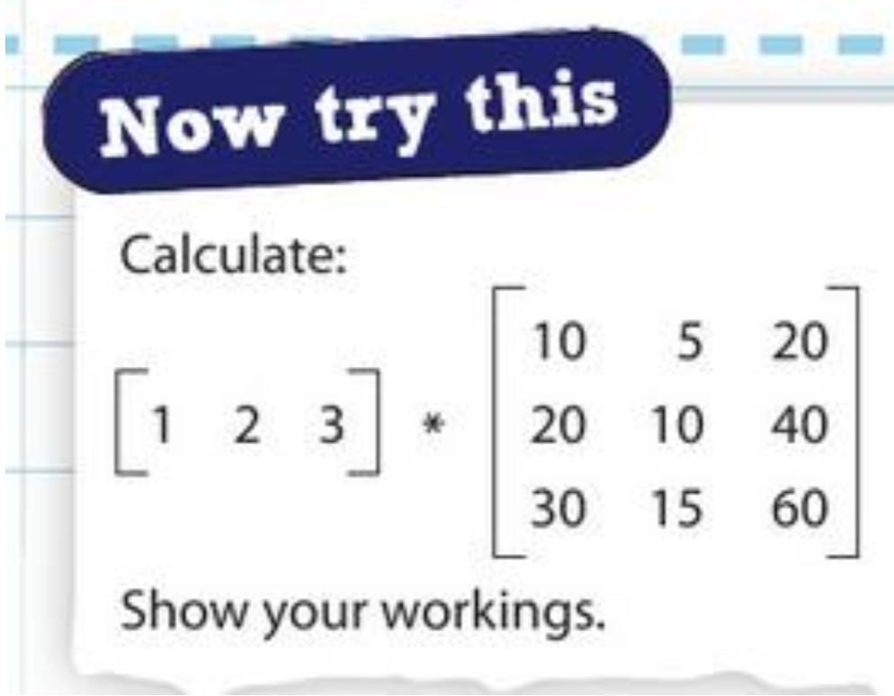
Multiplication

Matrix multiplication is challenging!
You can see these aren’t the same size: that’s fine. We first have to rotate the first matrix by 90 degrees.
2     12 14 15
3  x   5  6  6
4      7  9  8
We then look at the first column. We take the first item in the left matrix (2) and multiply it by the first item in the other matrix’s first column (12). 2 x 12 = 24.
After, we move to the next values down in both matrices: 3 x 5 = 15.
We repeat this until the end of the column, where we then go to the top of the next column and start from the beginning.
After, we should be left with this:
2     12 14 15     24 28 30
3  x   5  6  6  =  15 18 18
4      7  9  8     28 36 32
Our final step is to total up the columns to finish with:
24 + 15 + 28 = 67
28 + 18 + 36 = 82
30 + 18 + 32 = 80
Which gives us a final answer of…
[ 67 82 80 ]
Question


